Decoding Building Energy Patterns

The Role of Similarity Metrics in Clustering

In the built environment, understanding how energy is consumed is crucial for driving efficiency and sustainability. Clustering building energy data helps us identify patterns and trends that reveal where optimization opportunities lie.

Clustering is a machine learning technique used to segmenting data into meaningful groups. It's a type of unsupervised learning, meaning it works with unlabeled data and does not require predefined categories. The goal of clustering is to discover natural groupings or patterns in the data, which can then be used for further analysis or decision-making.

By grouping similar energy usage behaviors, we can better understand the dynamics of a building, from peak usage times to the impact of occupancy on energy demand. This understanding is crucial for reducing costs and enhancing sustainability. For example, if a cluster reveals that certain times of the day consistently see lower energy usage, it might be possible to reduce HVAC operation during those periods without compromising comfort. Conversely, identifying peak times can help in scheduling energy-intensive tasks more efficiently.

Clustering time or clustering activity? This is the question

As mentioned earlier, clustering is a starting point for gathering information about a building, often providing an opportunity to discuss the results with stakeholders. Depending on the objective, clusters can consist of days that follow a certain trend or days when specific events occur at particular times.

In my experience, a building's electricity consumption is primarily influenced by two factors: occupancy/human activity and external disturbances (such as temperature, humidity, and solar radiation). Time is often used as a proxy to observe the contribution of these factors, though they behave quite differently. Occupancy is inherently stochastic and challenging to predict, especially in residential buildings, while external disturbances are more predictable, though still subject to uncertainties.

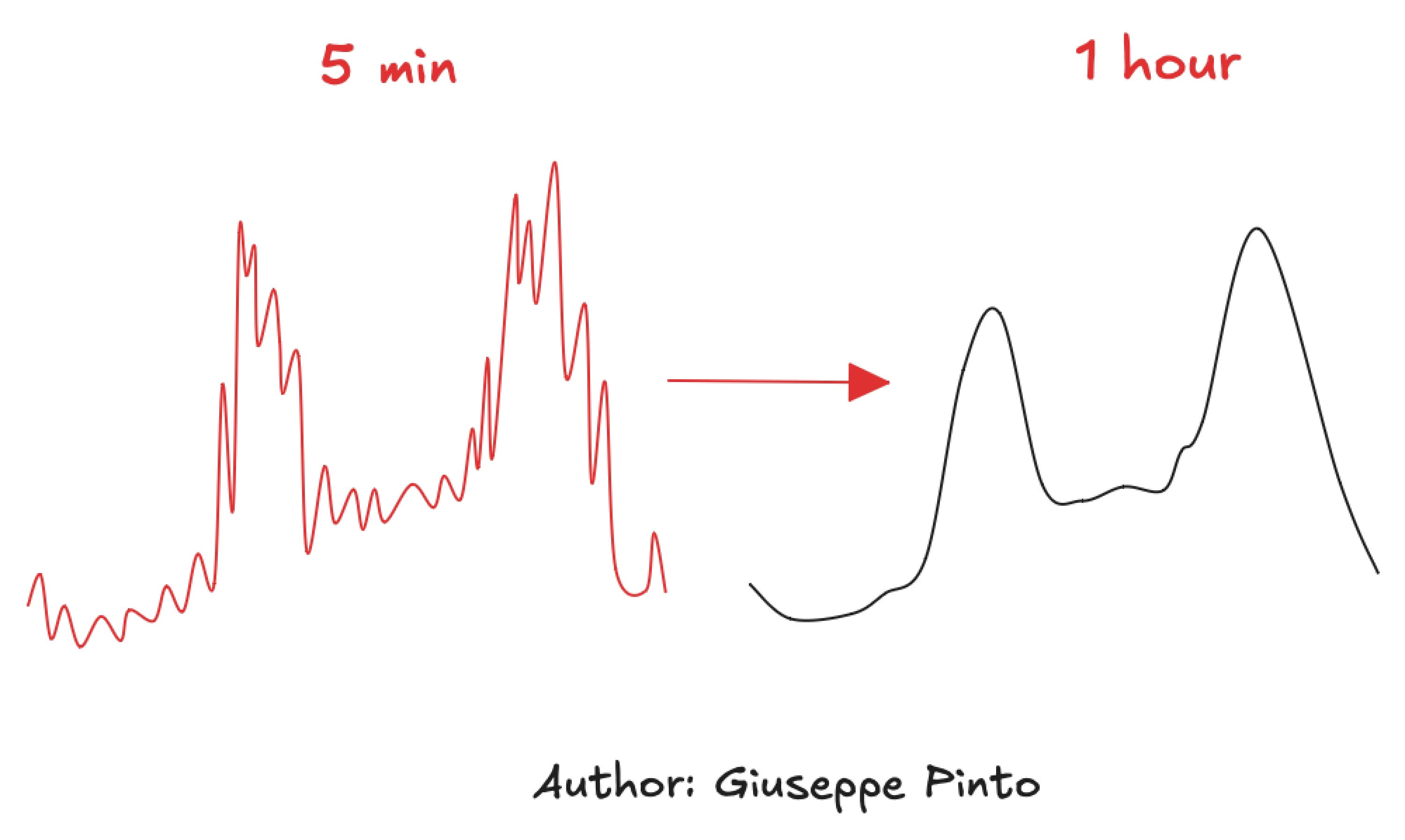
As a result, when analyzing a time series of electricity consumption, we observe the interaction between these two factors, which generates significant volatility over time. One way to reduce this volatility is by aggregating the data to a level that still preserves the necessary information—usually from 15-minute intervals to 1-hour intervals. This provides a first level of smoothing that makes pattern identification easier. For example, if your goal is to identify patterns for demand response with 15-minute granularity, that should be your upper limit. However, for now, we'll focus on the 1-hour interval.

Now that we have aggregated the time series, it's time to identify the major patterns by clustering the data. Some of the most popular clustering algorithms include K-means, hierarchical clustering, self-organizing maps, and density-based scan (DBSCAN). For this article, we'll focus on K-means, as it is likely the most well-known."

K-means

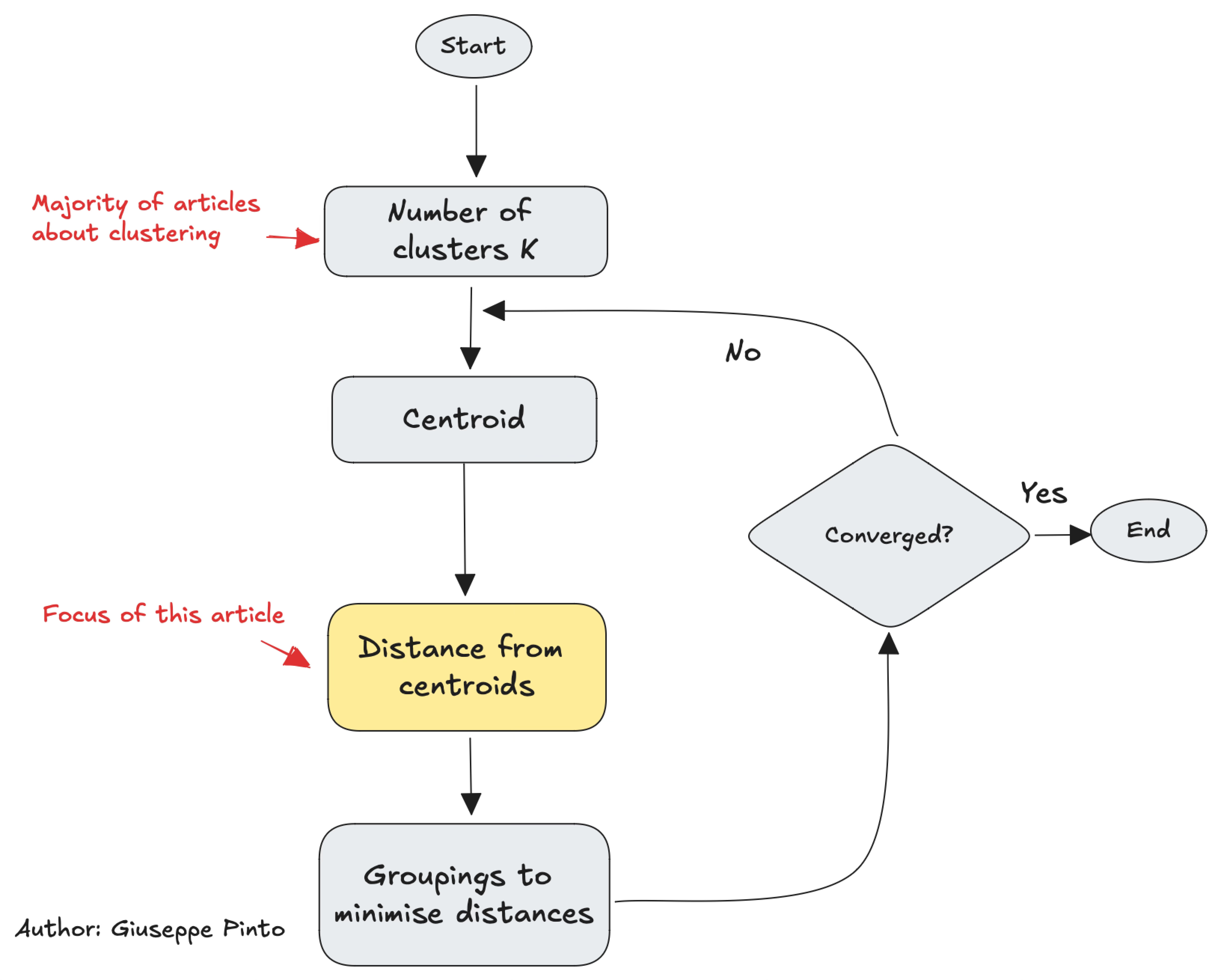
K-Means is a popular clustering algorithm that partitions data into a predefined number of clusters (K) by minimizing the variance within each cluster. It works by assigning data points to the nearest cluster center, recalculating the center based on the assigned points, and repeating this process until the clusters stabilize.

In case you need a refresh on how the algorithm works, here is a flowchart.

While there are dozens of articles on how to choose “K”¹, the most famous hyper-parameter of the algorithm, little attention is devoted to the distance used to evaluate the cluster centroids.

Clustering distance metrics: Euclidean vs DTW

Recalling what I wrote back, the biggest contributions to the electricity consumption comes from two sources: event-based (occupancy and human activity) or time-based (like external temperature, which often follows a sinusoidal pattern throughout the day). Given this, the choice of distance metrics becomes crucial, as it determines how profiles are grouped (by time of the day, or by event).

In this article, we will compare two specific metrics used to evaluate similarity between time series: Euclidian Distance and Dynamic Time Warping (DTW). Now, let’s take two instance of the previously drawn time series, where one is slightly shifted to the right and let’s evaluate the similarity between them.

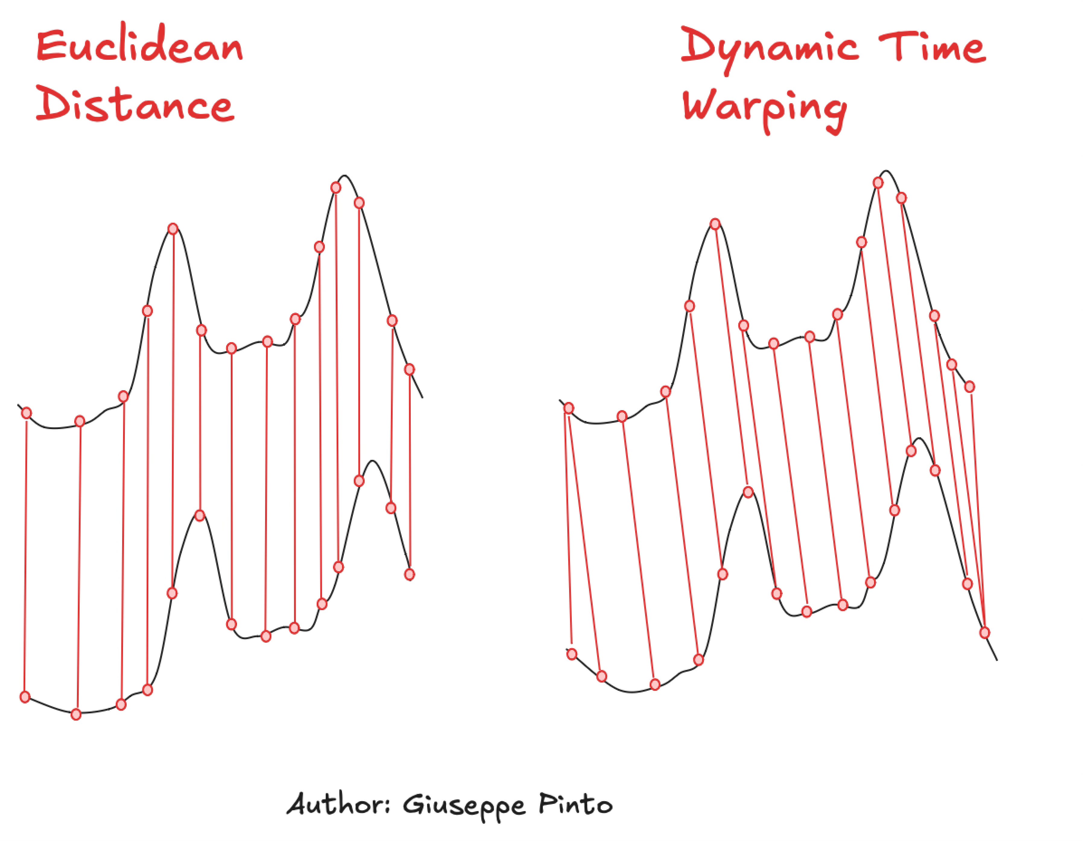
In the figure above, we are computing the similarity of the two time series using the Eucledean distance, left, and Dynamic Time Warping (right).

The similarity will be computed as the sum of distances between the matched features. You might notice that while the Euclidian distance looks for a “vertical difference”, using the same index position to compare two points, DTW matches distinctive patterns of the time series, allowing similar shapes to match even if they are out of phase or have varying speeds².

Residential house example

To show the importance of the similarity metric, consider a residential building with three distinct patterns:

• On Monday, Wednesday, and Friday, the energy usage follows a sinusoidal pattern.

• On Tuesday and Thursday, there are two or three peaks throughout the day.

• Over the weekend, the energy usage exhibits a flat behavior.

These profiles are not rigid and can vary in their start and end times. While the overall shape might be similar, phase shifts can occur. For example, a meeting running late might push lunch to a later time, or attending a gym class earlier could move up dinner time³.

When we perform K-means clustering, we need to set the number of clusters. In this case, choosing 3 clusters is a no-brainer, as we know there are primarily three distinct patterns, shown in the following picture.

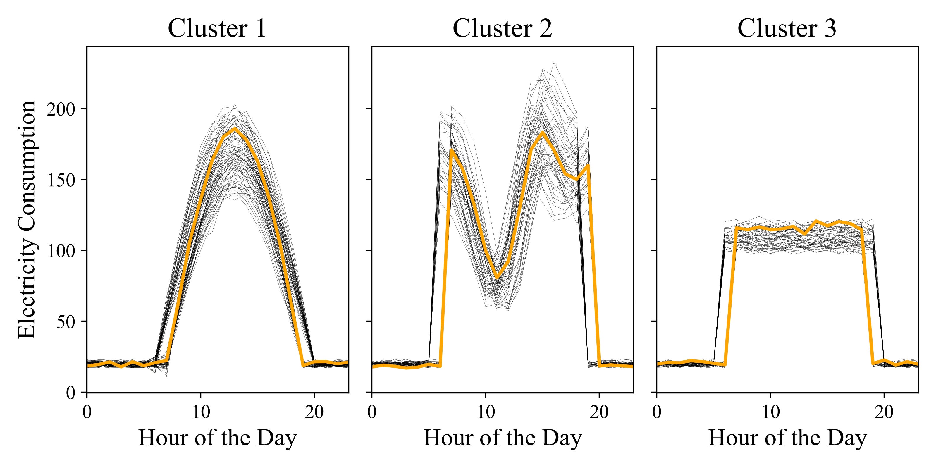
As you can see there are varying starting and ending time for each shape, while it is still easy to distinguish among them.

Clustering with default parameters

For the purpose of clustering, I like to use tslearn as it builds from sktlearn, but has more feature specifically tailored for time series analysis. Using TimeSeriesKMeans with the default for every hyper-parameter (except the number of clusters) will lead to evaluate the distance from centroids using Eucledean distance.

from tslearn.clustering import TimeSeriesKMeans
kmeans_eucledean = TimeSeriesKMeans(n_clusters=3).fit_predict(daily_data)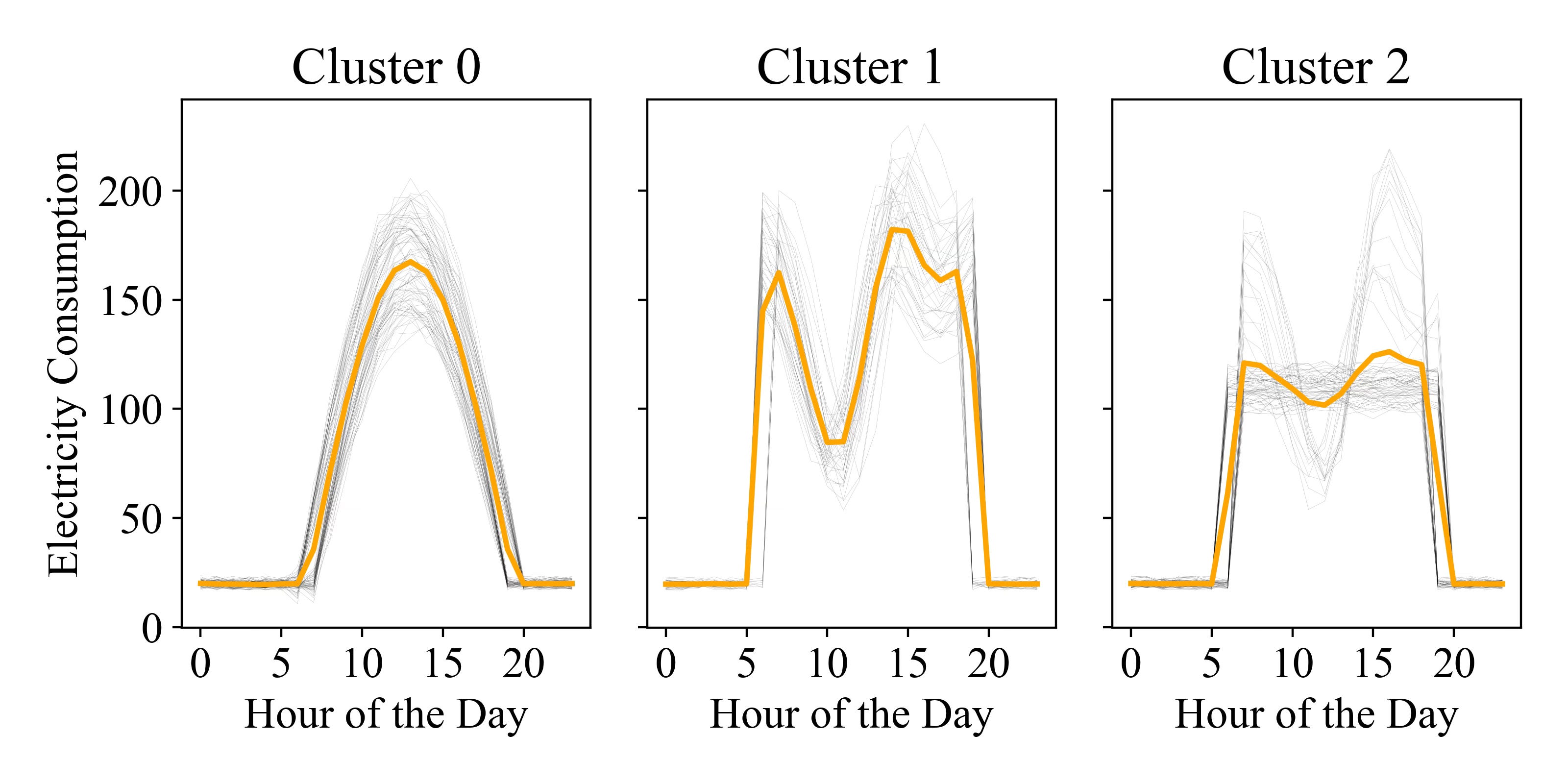

As you can see, the results are not satisfactory—the algorithm fails to identify the expected patterns. For example, Cluster 2 combines two distinct time series shapes, and the barycenter is not particularly representative of the time series within the cluster.

It's important to remember that, while it may seem obvious that there are three patterns based on the weekday, clustering a technique of unsupervised learning, and information such as day of the week represent a “label”, meaning we cannot use this information. This means the primary goal is to extract information without relying on a domain expert to visually inspect the data. Instead, we must 'trust' the algorithm to group the data in a way that reveals valuable insights.

Clustering with DTW

Given the poor results with Euclidean distance and observing that the time series seems more 'event-triggered' than time-based (as suggested by the shifts in the start and end times of the daily profiles), DTW might be a better choice. Fortunately, implementing this change requires just a 10-character adjustment in our code.

kmeans_dtw = TimeSeriesKMeans(n_clusters=3, metric="dtw").fit_predict(daily_data)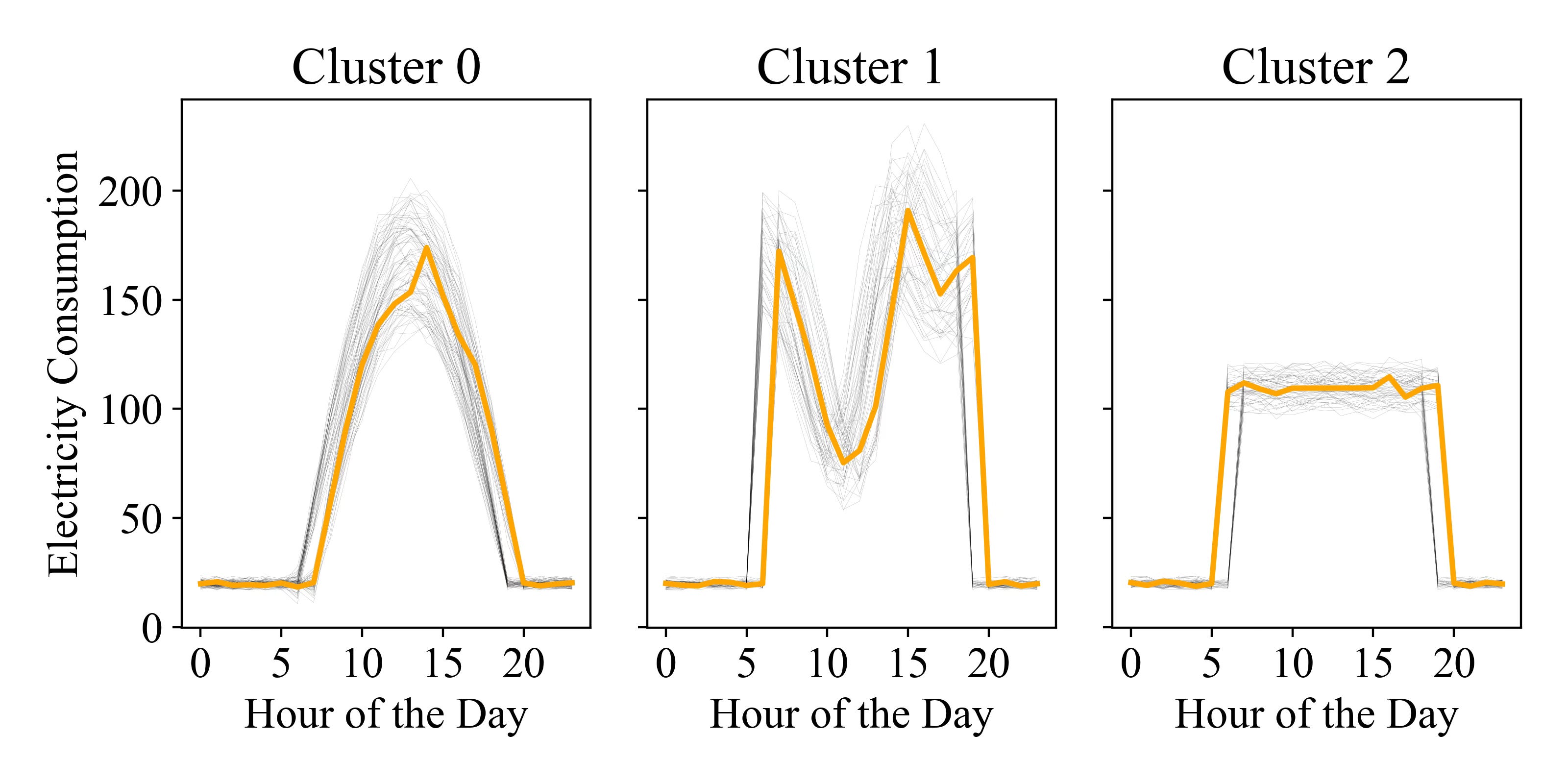

As shown in the picture above, the clustering now successfully identifies the three distinct shapes despite the lag, delivering the expected results.

Clustering analysis is typically performed during the data-exploration phase, and gaining a clear picture of the building’s behavior enables several important insights and actions for energy management:

• Load Forecasting and Management: Understanding the typical consumption patterns within each cluster helps utilities forecast demand more accurately and enables tailored management strategies to reduce costs or increase efficiency.

• Anomaly Detection: Buildings that deviate significantly from the centroid of their cluster can be flagged for further investigation, indicating potential inefficiencies, malfunctions, or unexpected changes in occupancy schedules.

• Targeted Energy Efficiency Programs: On a larger scale, comparing clusters of buildings with similar profiles enables targeted energy efficiency programs. This information allows energy providers to tailor energy-saving initiatives specific to the needs of each cluster.

Although DTW might seem superior, each domain has its own challenges, and the choice of distance metric has significant implications. Sometimes, using DTW can yield suboptimal results, particularly when the “time-vs-activity dance” is more subtle, and the factors share an even influence. In such cases, especially when dealing with energy management and the unpredictability of peak times, Euclidean distance might offer a different perspective on the problem.

My go-to approach is to start from DTW for residential profiles, where volatility is mainly driven by human activity, and to favour Euclidean distance when I know the patterns follow a more structured schedule (such as in a 9-to-5 office setting).

1. Here is one of my favourite articles about the number of cluster selection: https://towardsdatascience.com/are-you-still-using-the-elbow-method-5d271b3063bd

2. An excellent article dealing with DTW (from which I was inspired) is the following: https://rtavenar.github.io/blog/dtw.html

3. If you are wondering why these two specific examples, well, I generated the profile looking at my office vs smart working days.